Real and nominal value

Part of a series on
Economics
History Outline Index
Branches and classifications Applied Econometrics Heterodox International Micro / Macro Mainstream Mathematical Methodology Political JEL classification codes
Concepts, theory and techniques Economic systems Economic growth Market National accounting Experimental economics Computational economics Game theory Operations research Middle income trap Industrial complex
By application Agricultural Behavioral Business Cultural Demographic Development Digitization Ecological Education Engineering Environmental Evolutionary Expeditionary Feminist Financial Geographical Happiness Health Historical Humanistic Industrial organization Information Institutional Knowledge Labour Law Managerial Monetary Natural resource Organizational Participation Personnel Planning Policy Public Public choice / Social choice theory Regional Rural Service Socio Sociological Solidarity Statistics Urban Welfare
Notable economists de Mandeville Quesnay Smith Malthus Say Ricardo von Thünen List Bastiat Cournot Mill Gossen Marx Walras Jevons George Menger Marshall Edgeworth Clark Pareto von Böhm-Bawerk von Wieser Veblen Fisher Pigou Heckscher von Mises Schumpeter Keynes Knight Polanyi Frisch Sraffa Myrdal Hayek Kalecki Röpke Kuznets Tinbergen Robinson von Neumann Hicks Lange Leontief Galbraith Koopmans Schumacher Friedman Samuelson Simon Buchanan Arrow Baumol Solow Rothbard Greenspan Sowell Becker Ostrom Sen Lucas Stiglitz Thaler Hoppe Krugman Piketty more
Lists Glossary Economists Publications (journals) Schools
Business portal Money portal
v t e

In economics, nominal value refers to value measured in terms of absolute money amounts, whereas real value is considered and measured against the actual goods or services for which it can be exchanged at a given time. Real value takes into account inflation and the value of an asset in relation to its purchasing power.

In macroeconomics, the real gross domestic product compensates for inflation so economists can exclude inflation from growth figures, and see how much an economy actually grows. Nominal GDP would include inflation, and thus be higher.

Commodity bundles, price indices and inflation

A commodity bundle is a sample of goods, which is used to represent the sum total of goods across the economy to which the goods belong, for the purpose of comparison across different times (or locations).

At a single point of time, a commodity bundle consists of a list of goods, and each good in the list has a market price and a quantity. The market value of the good is the market price times the quantity at that point of time. The nominal value of the commodity bundle at a point of time is the total market value of the commodity bundle, depending on the market price, and the quantity, of each good in the commodity bundle which are current at the time.

A price index is the relative price of a commodity bundle. A price index can be measured over time, or at different locations or markets. If it is measured over time, it is a series of values ${\displaystyle P_{t}}$ over time ${\displaystyle t}$.

A time series price index is calculated relative to a base or reference date. ${\displaystyle P_{0}}$ is the value of the index at the base date. For example, if the base date is (the end of) 1992, ${\displaystyle P_{0}}$ is the value of the index at (the end of) 1992. The price index is typically normalized to start at 100 at the base date, so ${\displaystyle P_{0}}$ is set to 100.

The length of time between each value of ${\displaystyle t}$ and the next one, is normally constant regular time interval, such as a calendar year. ${\displaystyle P_{t}}$ is the value of the price index at time ${\displaystyle t}$ after the base date. ${\displaystyle P_{t}}$ equals 100 times the value of the commodity bundle at time ${\displaystyle t}$, divided by the value of the commodity bundle at the base date.

If the price of the commodity bundle has increased by one percent over the first period after the base date, then P₁ = 101.

The inflation rate ${\displaystyle i_{t}}$ between time ${\displaystyle t-1}$ and time ${\displaystyle t}$ is the change in the price index divided by the price index value at time ${\displaystyle t-1}$:

${\displaystyle i_{t}={\frac {P_{t}-P_{t-1}}{P_{t-1}}}}$

${\displaystyle ={\frac {P_{t}}{P_{t-1}}}-1}$

expressed as a percentage.

Real value

The nominal value of a commodity bundle tends to change over time. In contrast, by definition, the real value of the commodity bundle in aggregate remains the same over time. The real values of individual goods or commodities may rise or fall against each other, in relative terms, but a representative commodity bundle as a whole retains its real value as a constant from one period to the next.

Real values can for example be expressed in constant 1992 dollars, with the price level fixed 100 at the base date.

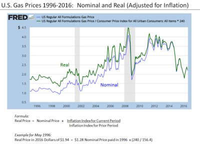
The price index is applied to adjust the nominal value ${\displaystyle Q}$ of a quantity, such as wages or total production, to obtain its real value. The real value is the value expressed in terms of purchasing power in the base year.

The index price divided by its base-year value ${\displaystyle P_{t}/P_{0}}$ gives the growth factor of the price index.

Real values can be found by dividing the nominal value by the growth factor of a price index. Using the price index growth factor as a divisor for converting a nominal value into a real value, the real value at time t relative to the base date is:

${\displaystyle {\frac {P_{0}\cdot Q_{t}}{P_{t}}}}$

Real growth rate

The real growth rate ${\displaystyle r_{t}}$ is the change in a nominal quantity ${\displaystyle Q_{t}}$ in real terms since the previous date ${\displaystyle t-1}$. It measures by how much the buying power of the quantity has changed over a single period.

${\displaystyle r_{t}={\frac {P_{0}\cdot Q_{t}}{P_{t}}}{\Bigg /}{\frac {P_{0}\cdot Q_{t-1}}{P_{t-1}}}-1}$

${\displaystyle ={\frac {P_{t-1}\cdot Q_{t}}{P_{t}\cdot Q_{t-1}}}-1}$

${\displaystyle ={\frac {Q_{t}}{Q_{t-1}}}({\frac {P_{t}}{P_{t-1}}})^{-1}-1}$

${\displaystyle ={\frac {1+g_{t}}{1+i_{t}}}-1}$

where ${\displaystyle g_{t}}$ is the nominal growth rate of ${\displaystyle Q_{t}}$, and ${\displaystyle i_{t}}$ is the inflation rate.

${\displaystyle 1+r_{t}={\frac {1+g_{t}}{1+i_{t}}}}$

For values of ${\displaystyle i_{t}}$ between −1 and 1 (i.e. ±100 percent), we have the Taylor series

${\displaystyle (1+i_{t})^{-1}=1-i_{t}+i_{t}^{2}-i_{t}^{3}+...}$

so

${\displaystyle 1+r_{t}=(1+g_{t})(1-i_{t}+i_{t}^{2}-i_{t}^{3}+...)}$

${\displaystyle =1+g_{t}-i_{t}-g_{t}i_{t}+i_{t}^{2}+{\text{higher order terms.}}}$

Hence as a first-order (i.e. linear) approximation,

${\displaystyle r_{t}=g_{t}-i_{t}}$

Real wages and real gross domestic products

The bundle of goods used to measure the Consumer Price Index (CPI) is applicable to consumers. So for wage earners as consumers, an appropriate way to measure real wages (the buying power of wages) is to divide the nominal wage (after-tax) by the growth factor in the CPI.

Gross domestic product (GDP) is a measure of aggregate output. Nominal GDP in a particular period reflects prices that were current at the time, whereas real GDP compensates for inflation. Price indices and the U.S. National Income and Product Accounts are constructed from bundles of commodities and their respective prices. In the case of GDP, a suitable price index is the GDP price index. In the U.S. National Income and Product Accounts, nominal GDP is called GDP in current dollars (that is, in prices current for each designated year), and real GDP is called GDP in [base-year] dollars (that is, in dollars that can purchase the same quantity of commodities as in the base year).

Example

If for years 1 and 2 (possibly a span of 20 years apart), the nominal wage and price level P of goods are respectively nominal wage rate: $10 in year 1 and $16 in year 2 price level: 1.00 in year 1 and 1.333 in year 2, then real wages using year 1 as the base year are respectively: $10 (= $10/1.00) in year 1 and $12 (= $16/1.333) in year 2. The real wage each year measures the buying power of the hourly wage in common terms. In this example, the real wage rate increased by 20 percent, meaning that an hour's wage would buy 20% more goods in year 2 compared with year 1.

Real interest rates

As was shown in the section above on the real growth rate,

${\displaystyle 1+r_{t}={\frac {1+g_{t}}{1+i_{t}}}}$

where

${\displaystyle r_{t}}$ is the rate of increase of a quantity in real terms,

${\displaystyle g_{t}}$ is the rate of increase of the same quantity in nominal terms, and

${\displaystyle i_{t}}$ is the rate of inflation,

and as a first-order approximation,

${\displaystyle r_{t}=g_{t}-i_{t}.}$

In the case where the growing quantity is a financial asset, ${\displaystyle g_{t}}$ is a nominal interest rate and ${\displaystyle r_{t}}$ is the corresponding real interest rate; the first-order approximation ${\displaystyle r_{t}=g_{t}-i_{t}}$ is known as the Fisher equation.^[1]

Looking back into the past, the ex post real interest rate is approximately the historical nominal interest rate minus inflation. Looking forward into the future, the expected real interest rate is approximately the nominal interest rate minus the expected inflation rate.

Cross-sectional comparison

Not only time-series data, as above, but also cross-sectional data which depends on prices which may vary geographically for example, can be adjusted in a similar way. For example, the total value of a good produced in a region of a country depends on both the amount and the price. To compare the output of different regions, the nominal output in a region can be adjusted by repricing the goods at common or average prices.

See also

Notes

References

• Diewert, W. E. (2008) [1987]. "Index Numbers". The New Palgrave Dictionary of Economics (2nd ed.). pp. 1–32. doi:10.1057/978-1-349-95121-5_940-2. ISBN 978-1-349-95121-5.
• O'Donnell, R. (1987). "Real and Nominal Quantities". The New Palgrave: A Dictionary of Economics. Vol. v. 4. pp. 97–98. (Adam Smith's early distinction vindicated)
• Sen, Amartya (1979). "The Welfare Basis of Real Income Comparisons: A Survey". Journal of Economic Literature. 17 (1): 1–45. JSTOR 2723639.
• Usher, D. (1987). "Real Income". The New Palgrave: A Dictionary of Economics. Vol. v. 4. pp. 104–05.

External links

• DataBasics: Deflating Nominal Values to Real Values from Federal Reserve Bank of Dallas
• CPI Inflation Calculator from U.S. Bureau of Labor Statistics